Scanning Near-Field Optical Microscopy

This tutorial is for the SNOM model NT-MDT NOVA.

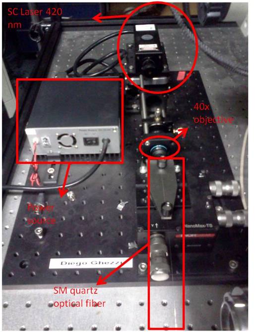
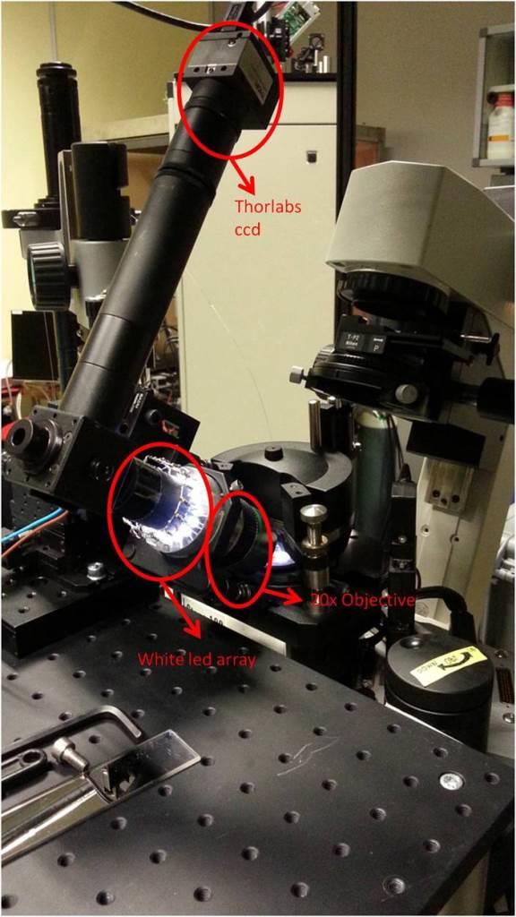
The setup consists in a microscope column with a 20x objective (reflection) and a xy piezo stage to move the sample. On top of it there is a scanning head in which we can insert the snom fiber; the head, and consequently the optical fiber, is controlled with a xyz piezo controller. The fiber is fed with a blue laser (SDL-473-100 T) coupled by a 40x objective. The quartz fiber is tapered and coated with aluminum, with a final aperture of 100 nm.

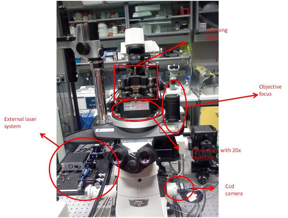
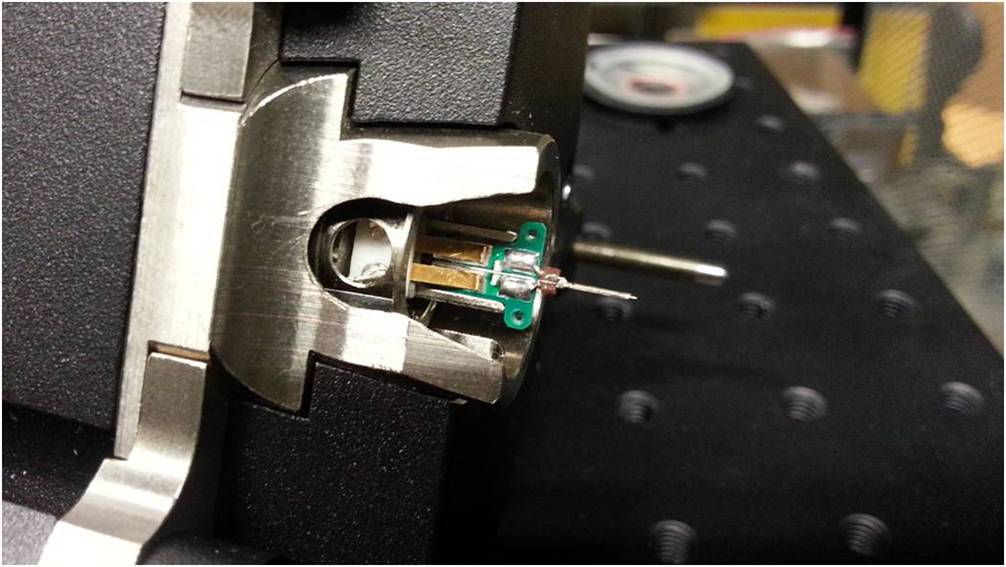
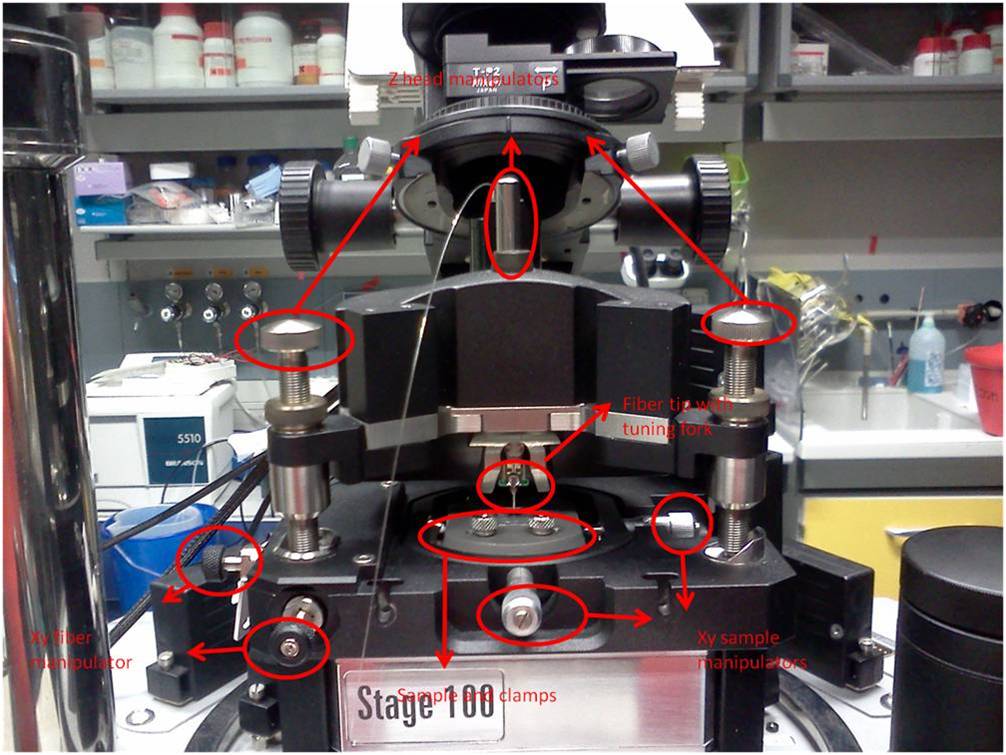
The NT-MDT uses special SNOM fibers (NT-MDT MF 112-NTF), obtained from Nufern 460-HP, single mode (core 2.5 µm) with a transmission coefficient around 10^-4. Each fiber is provided with a fork glued near the tip, with two electrodes matching the aperture in the scanning head. The fiber is inserted in the head from the bottom, until it firmly fits in the proper aperture and the metallization matches.

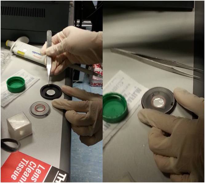
The other fiber's end must be properly stripped and cut for the coupling with the external laser. The fiber end will be kept in position with magnetic holders. The alignment procedure consists in maximizing the laser transmission inside the fiber checking the intensity of the scattered light along the fiber or looking for a little blue light exiting from the fiber tip.

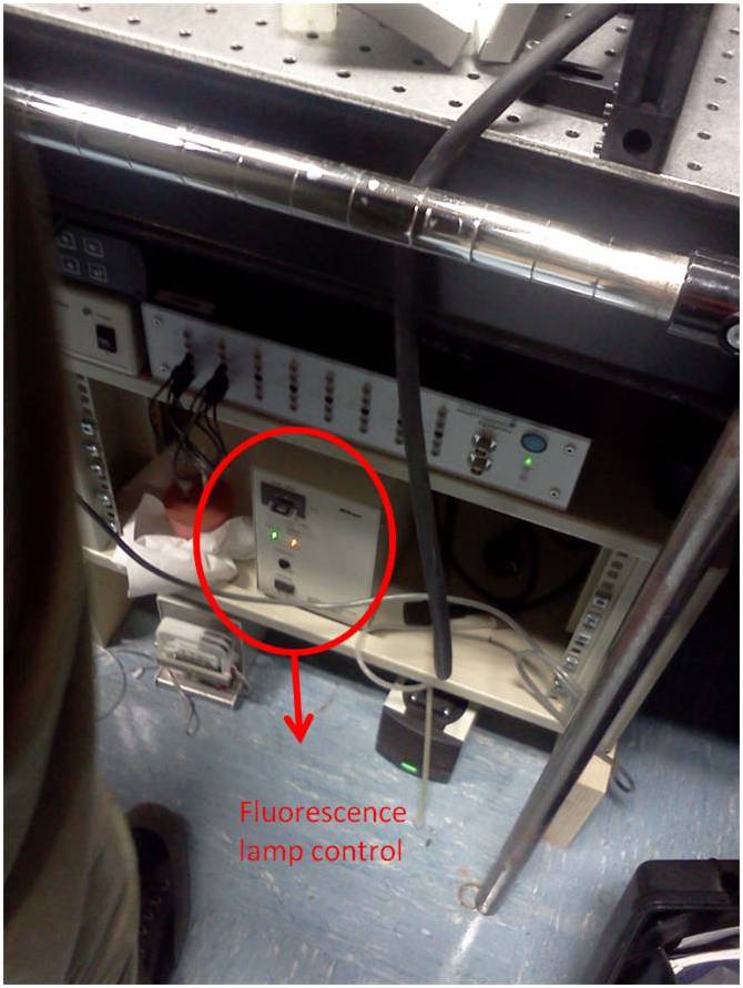
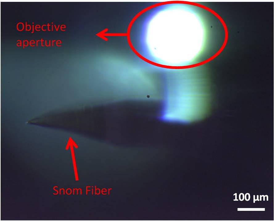
Once the described above alignment procedure is completed, it requires to align the fiber to the 20x objective in the piezo stage. This is a crucial task, since we don't have a clear view of the fiber position respect to the objective. In fact, since the scanning head doesn't allow a direct illumination from the top, we had to rely on a fluorescence lamp for illuminating the sample and the tip from the bottom. In this way the light emerging from the objective could be matched with the blue light exiting from the fiber tip.

Unfortunately it seems that the illumination path of the fluorescence lamp is slightly tilted respect to the objective axis, making the alignment more difficult. So we decided to install a second CCD in reflection mode; that is a Thorlabs usb-camera with a Mitutoyo APO 20X per DARK-BRIGTH mode with ultra long working distance > 30mm, mounted on a tilted micromanipulator.

So, in order to have a rough alignment, we put on the stage a dry sample, that is a round coverslip in a chamber for liquids and we fixed it in position with double-tape.

We switched on the controllers and we launched the NOVA SNOM software. To the left of the main window there's a tiny icon representing some boxes: clicking it will open the oscillogaph control. Selecting Video -> Play the transmission camera is turned on. The optical tube lenght of the microscope objectives was adjusted to correctly image the surface of the sample. Then we put the scanning head on the stage, so we first protruded the rear leg so that the tip did not touch the sample. The front legs must be at the same level. To protrude the legs, they must be rotated clockwise. Once the head is in position, the rear leg can be lowered manually to a distance of 1 mm circa from the sample. At this point the head should be horizontal, otherwise we have to act on the front legs.

The transmission camera has a field of view of 80 µm and a depth of view of a few microns, so it's really difficult to check the position of the tip respect to the objective and it can be done only when the tip is really close to the sample. With the external CCD system, instead, we can obtain field of view up to 1mm circa and it's easier to spot the light exiting from the objective. The fiber can thus be moved towards the spot for an easier alignment.

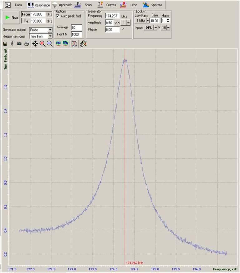
After the rough alignment, we switched on the controllers for the fork; they are located on the desktop case. We searched for the resonance frequency of the tip. For the tips provided by NT-MDT, the first peak of resonance is around 33 kHz, but is preferable to use a harmonic at around 185 kHz for more stability. The goal is to obtain a well defined, sharp and narrow peak of at least 1 nA (but less than 42 nA to avoid saturation). So in the Resonance menu we put a frequency range between 170 and 190 kHz and we modified the amplitude and gain parameters. Typical values in air are 0.3V x0.1 Amplitude and 5 Gain. If possible, the gain has to be decreased to reduce the noise. Once the Lock in is set, we started the approaching of the tip to the sample. So in the Approach menu we set the Set Point to the value of the resonant peak (indicated aside). Then we pressed the icon of the Feedback loop FB and we lowered the set point until the approaching bar, located at the bottom of the main window, was completely filled. Then the approaching speed had to be set; a suitable speed for a new tip will be 18, then we can increase to 20 when it gets older. We clicked on Landing and the tip moved down towards the sample. There is the possibility that this procedure doesn't come to a good ending, so we have to remove the Feedback Loop and repeat everything from the Resonance step. Eventually the Landing will succeed, so the tip will be near enough to the sample (some atoms away) to do snom or shear force topography measurements. We can see that the landing is complete, a part from the green writing, also from the oscillograph measurement that becomes more noisy. Then we had to remove the Feedback loop to put the tip to a safe distance and go again to the Spectra menu. From here we can choose whether to move the tip or the sample to locate the structure to test. We can also use the manual translation with the screws on the instrumentation. If the tip is well centered on the objective, its shadow should be visible; otherwise we have to move the tip to the center of the objective. Once the tip is visible and the structures of interest can be seen, we move to the Scan menu. From here we can choose which scanning modality we want to perform, that is SNOM or shear force. In the tutorial we practiced on the shear force scanning, we set the frequency or speed of scanning and the area of interest. Depending on the structure, we can choose the scanning direction more suitable. So we put again the feedback loop and we start the scan. During the scan is possible to modify the set point (lowering it will decrease the noise) and the feedback gain (same). Basically, we have to avoid the spikes on the graph (too much pressure) but also a signal too clean, almost sinusoidal (almost no contact). When the scan ends (or when we decide to end it) we can save the image in a nt-mdt format or export it in a common format. To rapidly etract the tip we can use the « icon, while to rapidly approach (be careful!) we can select » and put the amount in mm.

Test in wet condition

After the test with the dry sample, we tried a wet approach. Here there are some problems. The first is that the electrodes mustn't touch the water, so it is recommended to have just a thin layer of liquid over the sample to be tested. The other problem is that the resonance peak will change quite fast flowing the drying of the liquid. Moreover, the intensity of the resonance peak will be lower for the higher shear in the liquid environment. With a rigid sample in liquid, the scanning can still be performed. But neurons cannot be distinguished very well from water in term of density, so the soft cell is pushed by the tip towards the glass, with a risk of breaking the glass or the tip (and obviously exerting a mechanical pressure on the neuron). Also, the neuronal parts can attach to the tip, thus altering he scanning. So a scanning seems not possible, but it is still possible to approach manually the tip to a neuron and keep it in position to exploit a near field excitation. Neurons growth on a glass coverslip were fixed and than put in the sample holder with 200 µl of PBS, obtaining a film of liquid thin enough to touch only the fiber tip but not the electrodes.

Via software we moved the tip in the liquid and we performed a resonance measurement. Because of the different medium respect to the dry condition, the parameters were changed, so we used an amplitude of oscillation of 0.5V.

The peak of resonance was blue-shifted respect to the dry condition and changed in time because of the drying of the liquid, but slowly enough to be followed by the following resonance measurement. So we moved the sample and the objective turret to focus the soma of a neuron. After that we started a recursive approaching, doing alternatively a resonance measurement and a landing to keep track of the shift in resonance. Eventually the fiber tip, and the blue light exiting from it, was visible in the transmission CCD camera, so we could move the tip in axis with the soma and end the landing process on the cell itself.

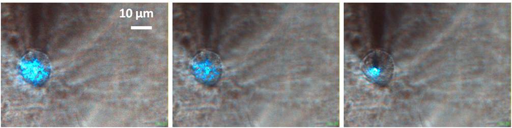
Again the landing must be controlled, otherwise the tip will just dig into the membrane until it feels the glass underneath. A good way to decrease the pressure was to reduce the feedback gain FB to 0.05 to have a slower approach. Also, after the landing, we retracted the tip step by step in order to reduce the pressure on the membrane. This procedure gave us the possibility to keep the tip in contact with the cell or slightly above. Unfortunately, the smallest distance that can be controlled in the z axis is 10 µm, so we don't have a precise value for the distance between the tip and the membrane. Anyway, also from the dimension of the blue spot, it can be understood when we are in proximity.

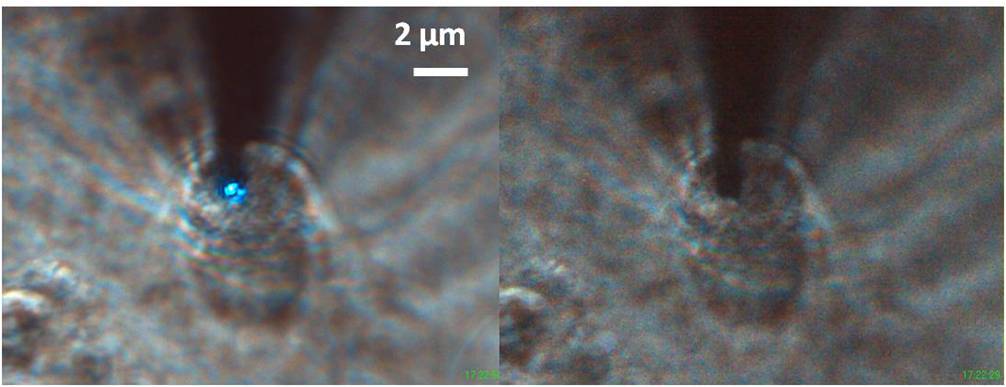
We tried to perform a topographic scanning, to see whether the contact could be maintained, and we obtained it. During the scanning of the sample, the membrane follows the tip but we have avoided to break it.

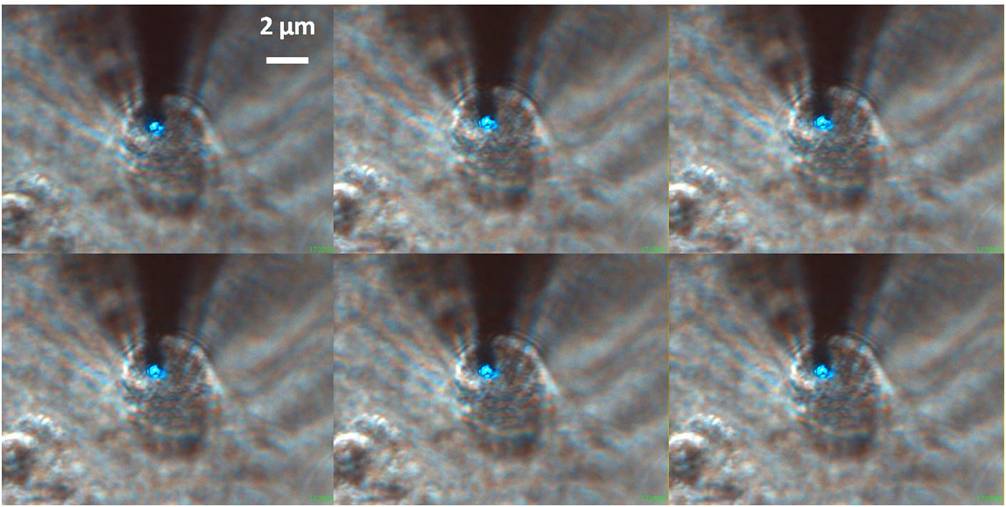
We did the approaching on three different cells, achieving always a good contact.